WebGL Based CNN
This has been a 3 week slog, and only in the last couple days have I decided that it is a somewhat worthy pursuit. I’m basically not sure about anything regarding this little project and until I have a demo which does something, and does it how I expect it should, will I be sure that it’s worth it.
For now I’m seeing this write up as a chance for me to give it a once over with a fine-tooth comb and see if I’ve missed anything. As it stands, and as a TL;DR: I believe this WebGL based CNN is performing 2D convolutions on an input tensor to downscale and then upscale, with varying numbers of filters, and performing this much faster than the equivalent model running on the web using Tensorflow JS.
Why do this again?
The key motivation behind this is to address the performance issues that are unavoidable with Tensorflow JS. Internally TF-JS uses a GPGPU approach to perform the computations in a neural network which involves loading data into buffers and reading those buffers a bunch of times at inference time. It works really well, but this approach is always going to hit a performance limit: there is only so fast that WebGL or some equivalent engine can read to or from a buffer.
So the approach I’m taking with this is to load all the data into buffers at setup-time, and then to only access this data to display to the screen; all computation happens in the shader programs which pass data through the computational graph using frame buffers.
Its specific purpose is to run an Autoencoder model like the generator used in the Pix2Pix model and only really needs to perform one task: 2D convolutions. I’m not even going to say it needs to perform deconvolutions or 2D transpose convolutions as they are sometimes called for reasons I’ll go through later.
Things to Note
TODO:
- Define: tensor, filter, kernal
- Explain how data is stored in 2D vectors, eg 4 filters being defined by
vec2(2)
The Approach
NB: I would quite like to make some nice graphics which will help explain this in a visual way, but that’s not high on my priority list right now. So this might be quite wordy, with some borrowed graphics, or photos of sketches.
Most/all of the actual maths-y code will be in the fragment shader. The purpose of the fragment shader is essentially to colour the pixels of the screen (or fragments in shader land) based on the information it has been provided. That information may well be a 3D scene with perspective and overlapping objects and fog and lighting etc.. but in our case it’s quite simple, it will be provided with two textures as input: 1. the incoming tensor and 2. the filter kernals to be used in the convolution.
Simple enough, but there are a number of challenges posed already. Fragment shader code is a single script which is used for every fragment to be rendered. If you are rendering to a screen of 100x80 pixels, and you are working at full resolution, then the fragment shader code will run 100x80 times, once for each fragment, in unison. A given fragment has a coordinate which is called gl_FragCoord in GLSL. gl_FragCoord coresponds to where it lands in the output image, and it is this coordinate which must become the reference point for all calculations. The temptation to think of a for loop iterating over pixel by pixel is certainly there, but this is misleading as you do do not have that same indexing capability; each fragment is all alone in relation to all other fragments.
The first issue here is that our input data is a tensor, and a tensor in a CNN is often thought of as a cube, as shown in the canonical image of the AlexNet architecture:
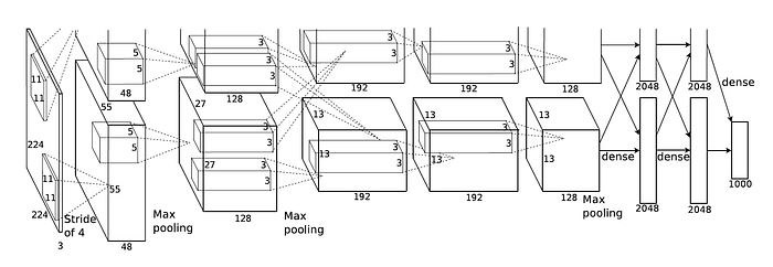
Tensors of such shape are easy to handle with the incredible Python library Numpy is essentially the backbone of all data science ever. Creating a tensor of dimensions 27x27x128 is as easy as numpy.zeros((27, 27, 128)). In fragment shader land we have to work in only two dimensions. So we need to flatten this tensor out into a 2D image (a texture). The third dimension can be thought of as the number of layers of the same image but slightly different, just like an RGB image: RG and B are different layers of a single image which can be seperated and viewed as different images in their own right. An RGB image is a tensor of shape WxHx3, or WxHx{R,G,B}. The same can be said for a 27x27x128 tensor; 128 layers of some variation on a 27x27 matrix/image/whatever you wanna call it. So to immediately make this easier for us we are only ever going to use square numbers for the number of filters we use per layer, because it is the number of filters in a given layer which determines the depth of the outgoing tensor. Eg. look at the second layer in the AlexNet image above, the depth of that tensor is 48, that means they used 48 filters on the input image. By sticking to this rule we can easily spread out 16 filters into a 4x4 grid, or 64 filters in an 8x8 grid, and so on.
3D textures do exist in WebGL and are made easy to use in WebGL2, but a fragment shader can only ever output to a 2D image; 3D displays don’t exist just yet. We could put the data into a 3D texture but this would then require a call to
getBufferSubData()as the output would not go directly into a frame buffer.
[TODO: IMAGE - 3D tensor === 2D texture]
Each layer in our 3D output tensor is formed by convolving one filter across the whole input tensor - hence why the number of filters for a given layer in a CNN gives you the depth of the output tensor. So in our fragment shader based version, this means we need to sample the flattened input tensor at multiple points using the correct corresponding kernel in our filter, which is also falttened. Let’s take a simple example…
Our input tensor will be 8x8x4, our filter for that tensor needs to have the same depth in order to convolve every layer, so that will be 4x4x4, and we want and output tensor of shape 4x4x4, so we need 4 filters:
    Input Tensor:
       +--------+
      /        /|           1 Filter:
     /        / |            +----+
    +--------+  |           /    /|
    |        |  |          +----+ |  (x4)
    |        |  +         4|    | +
  8 |        | /           |    |/4
    |        |/ 4          +----+
    +--------+               4
        8
We will reshape the input tensor and filter to look like this (not the best ASCII art, but hopefully if you look back in a while this will be replaced by something better).
Input: 8x8x4           Filter: 4x4x4 (x4)
+--------+--------+    +--+--+      +--+--+      +
|        |        |    |     |      |     |
| [8x8]  | [8x8]  |    +[4x4]+      +[4x4]+
|        |        |    |     |      |     |
|        |        |    +--+--+      +--+--+      +
+--------+--------+
|        |        |
| [8x8]  | [8x8]  |
|        |        |    +--+--+      +--+--+      +
|        |        |    |     |      |     |
+--------+--------+    +[4x4]+      +[4x4]+
                       |     |      |     |
                       +--+--+      +--+--+      +


                       +     +      +     +      +
So to convolve the input tensor, we need to take the result of a 4x4 convolution at each equivalent point on the flattened input tensor.. This is one convolution:
Input: 8x8x4           Filter: 4x4x4 (x4)              Output: 4x4x4
+--------+--------+    +--+--+      +--+--+      +     +-----+--
|*       |*       |    |*    |*     |     |            |*    |
|        |        |    +     +      +     +            |     |
|        |        |    |     |      |     |            |     |
|        |        |    +--+--+      +--+--+      +     +-----+
+--------+--------+     *     *                        |
|*       |*       |
|        |        |
|        |        |    +--+--+      +--+--+      +
|        |        |    |     |      |     |
+--------+--------+    +     +      +     +
                       |     |      |     |
                       +--+--+      +--+--+      +


                       +     +      +     +      +
Hopefully you can see that one convolution involves one filter which convolves every layer of the input tensor and every layer of that filter. These values are summed and become one layer in the output tensor. This is repeated for each filter to build up the output tensor:
Input: 8x8x4           Filter: 4x4x4 (x4)              Output: 4x4x4
+--------+--------+    +--+--+      +--+--+      +     +-----+-----+
|@       |@       |    |     |      |     |            |     |     |
|        |        |    +     +      +     +            |     |     |
|        |        |    |     |      |     |            |     |     |
|        |        |    +--+--+      +--+--+      +     +-----+-----+
+--------+--------+                                    |     |@    |
|@       |@       |                                    |     |     |
|        |        |                                    |     |     |
|        |        |    +--+--+      +--+--+      +     +-----------+
|        |        |    |     |      |@    |@
+--------+--------+    +     +      +     +
                       |     |      |     |
                       +--+--+      +--+--+      +
                                     @     @


                       +     +      +     +      +
So that output tensor is now a 2D image which WebGL renders into a framebuffer (offscreen, nice and quick) for us which gets stored in a texture, which we can pass into the next convolution shader program. That is the basic structure of how this system works! Simple in theory, but as you may notice, as the depth of the tensors increases, the layout of the filters quickly becomes confusing.. Take a layer which receives an input tensor of depth 8 and has 16 filters, each one of those filters being 8 layers deep.. Your filter texture then has the structure 4x4x8x16… I’ll try this in ASCII, might be a laugh:
Filters as one texture:

4x4 Kernal
 |
 |  x8
 |  |      x16
 |  |       |
+-+-+-+-+-------+-------+-------+
| | | | |       |       |       |
+-+-+-+-+       |       |       |
| | | | |       |       |       |
+-+-+-+-+       |       |       |
| | | | |       |       |       |
+-+-+-+-+       |       |       |
| | | | |       |       |       |
+-+-+-+-+-------+-------+-------+
|       |       |       |       |
|       |       |       |       |
|       |       |       |       |
|       |       |       |       |
|       |       |       |       |
|       |       |       |       |
|       |       |       |       |
+-------+-------+-------+-------+
|       |       |       |       |
|       |       |       |       |
|       |       |       |       |
|       |       |       |       |
|       |       |       |       |
|       |       |       |       |
|       |       |       |       |
+-------+-------+-------+-------+
|       |       |       |       |
|       |       |       |       |
|       |       |       |       |
|       |       |       |       |
|       |       |       |       |
|       |       |       |       |
|       |       |       |       |
+-------+-------+-------+-------+
Accessing the Right Values
So how to we do this awkward indexing in the fragment shader? Numbers in shader programs are generally normalised so that they are in the range [0, 1]. So thinking in 1D for a second, and range of [0,4] is normalised to a range of [0,1] in 4 intervals:
[0, 1, 2, 3, 4) --> [0.0, 0.25, 0.5, 0.75, 1.0)
The square brackets
[ ]mean the values are inclusive, and parentheses( )mean the values are exclusive. So the range[0,4)here means the 4 is excluded meaning the range is in fact[0, 1, 2, 3].
In the example we were using above, we know the output size will be 4x4, and there will be 4 of them, so the whole output image size is 8x8.
[TODO: Image - 2D image with dimensions showing the above]
What we are trying to do is find a range of numbers, based on gl_FragCoord that helps us index the input texture. gl_FragCoord will be of the range [0, 8), but our output tensor is actually of the shape 4x4x4, so if we divide gl_FragCoord by the output shape in x and y we will get a number range of the right length and of the right number of steps to traverse the input texture… Might be a bit easier to show you, and fortunately what works in 1 dimension will work for 2, so lets stick with 1 for now:
gl_FragCoord.x / output_size == [0, 8) / 4 = [0, 2) in 8 intervals
We’ll store this in a variable called st for the sake of convention, and this becomes our reference coordinate:
vec2 st = gl_FragCoord.xy / u_output_size; // [0, 8) / 4 --> [0, 2)
Our input texture is of the size 8x8x4, or 16x16. So to index the values in the top left layer of our tensor, we can take the fract() of st which basically takes the values after the decimal place in a floating point number: fract(1.567) == 0.567. This effectively gives us 2 number ranges of [0, 1), based on st:
[0, 2) in 8 intervals == [0, 1) in 4 intervals.. twice
Perhaps you’ve noticed something weird about this (or you’re completely lost already).. Our input tensor is of shape 8x8x4… so why do we want a range of values in 4 intervals and not 8? Well, we are trying to match the generator of the Pix2Pix model which downsamples an image without maxpooling. One way to do this is to use kernals of size 4x4, and use a stride of 2. By convolving over an input tensor at half it’s with and height, we acheive a stride of 2! So that saves quite a bit of calculating for us.
There is one last consideration based on how GLSL deals with textures we need to consider. The overall dimensions of a textrure are always [0, 1), so currently we would be spanning the entire with of the input tensor. So we can divide st by the depth of the input tensor (or the number of filters in the previous layer) to shrink the range [0,1) down to (in this case) [0, 0.5).
Input: 8x8x4 (texture)

0       0.5       1
+--------+--------+
|        |        |
|        |        |
|        |        |
|        |        |
+--------+--------+
|        |        |
|        |        |
|        |        |
|        |        |
+--------+--------+
I’m calling this input texture coord input_st:
vec2 input_st = fract(st) / u_num_filters_prev; // fract(0 -> 4) / 2 = 0 -> 0.5
Next we need a value to index the right filter. In this case we have 4 filters, but the number of filters can vary. All we want to do right now is “select” the right filter (in a way) by getting the upper left hand coordinate of the right filter. To do that we can take the floor() of st which discard the value of a floating point number after the decimal place (the opposite of fract()). In this example floor(st) gives us a value 0 or 1 depending on the value of gl_FragCoord. This is good as we have 4 filters we would get 4 possible values: 0,0, 1,0, 0,1 or 1,1. To get a useable value to access the texture we normalise by dividing by the number of filters.
We have 4 filters yes, but as we’re always working in 2D, the number of filters is actually represented by a
vec2like so:vec2(2, 2).
This is then stored in filter_offset:
vec2 filter_offset = floor(st) / u_num_filters; // floor(0 -> 2) / 2 = [0, 0.5, 1.0)
We’re getting somewhere…
The Convolution
We now have a way to index the input texture and the filters based on the current gl_FragCoord value. Next we need to get some loops involved - the first of which is to iterate over the number of filters:
for(float f_x=0.0; f_x<u_num_filters_prev.x; f_x+=1.0){
  for(float f_y=0.0; f_y<u_num_filters_prev.y; f_y+=1.0){
     vec2 layer = vec2(f_x, f_y);
     vec2 input_loc = input_st + (layer / u_num_filters_prev);
     vec2 filter_loc = filter_st + (layer * u_filter_texel_size * 4.0);

     /* ... */
  }
}
Remember that the number of layers is determined by the number of filters in the previous layer - that is the limit of our loop and store that as a vec2 called layer. The location sampled from the input texure, input_loc, is input_st plus the normalised value of layer.
We find the value of filter_loc by taking filter_st and adding layer scaled by the size of one kernel (u_filter_texel_size * 4.0).
A texel is the unit measurement of a texture, you can basically think of it as a pixel, but it’s not discrete like a pixel for now.
So as the double for loop iterates the lookup locations move across the input texture and the filters accordingly.
Inside this double loop we do a similar process but to iterate over the 4x4 kernel itself and get a single value which is the sum of the convolutions on each layer on the input tensor. First we need to define a function to actually get the values from the input texture and the filter, and multiply them. The function scales the offset based on the texel size of the input texture, or the filter texture.
float get(vec2 _input, vec2 _filter, vec2 _offset){
  float input_val  = texture(u_texture, _input + (_offset * u_input_texel_size)).r;
  float filter_val = texture(u_filter, _filter + (_offset * u_filter_texel_size)).r;

  return input_val * filter_val;
}
Instead of a nested for loop I just expanded the inner one to four seperate lines; to me that was easier to read. Our entire convolution loop looks like so:
float sum_row = 0.0;

for(float f_x=0.0; f_x<u_num_filters_prev.x; f_x+=1.0){
  for(float f_y=0.0; f_y<u_num_filters_prev.y; f_y+=1.0){
    vec2 layer = vec2(f_x, f_y);
    vec2 input_loc = input_st + (layer / u_num_filters_prev);
    vec2 filter_loc = filter_st + (layer * u_filter_texel_size * 4.0);

    for(float y=-1.5; y<2.0; y+=1.0){
       sum_row += get(input_loc, filter_loc, vec2(-1.5, y));
       sum_row += get(input_loc, filter_loc, vec2(-0.5, y));
       sum_row += get(input_loc, filter_loc, vec2( 0.5, y));
       sum_row += get(input_loc, filter_loc, vec2( 1.5, y));
    }
  }
}
Quite neat really.
Making Data
Upscaling, deconvolving, transpose convolutions are all names I’ve seen for the reverse process of a downscaling convolution. Basically making the input tensor bigger. The proces described above downsamples an image (in the x and y dimensions at least, if we only used one filter per layer then it would just make an image smaller by half each time), this is fine if our model was a classifier or something like that, but we want an image as an output so we need to scale those tensors back up to something we can ultimately render to the screen. This is the basic structure of an Autoencoder model and the generator of Pix2Pix:

Upscaling is a weird thing because you are, in one way or another, creating data. There are a few ways of approaching this, many are explained pretty well here. But this process in our fragment shader based approach is actually quite straightforward. Out upscaling shader program is nearly identical aside from the convolution loop:
for(float y=-0.75; y<1.0; y+=0.5){
  // Fractional Stride on input texture
  sum_row += get(input_loc, filter_loc, vec2(-0.75, y));
  sum_row += get(input_loc, filter_loc, vec2(-0.25, y));
  sum_row += get(input_loc, filter_loc, vec2( 0.25, y));
  sum_row += get(input_loc, filter_loc, vec2( 0.75, y));
}
Because we’re accessing texel values and not discrete pixels, we can sample whereever we want. So a fractional stride is prettty easy! We still don’t access data that wouldn’t otherwise be there in a normal array-like tensor, such as a Numpy array, but it quite easily solves this problem of injecting extra data into the larger output tensor.